
DenseNet -Densely Connected Convolutional Networks (CVPR 2017) 📑
CVPR 2017, Best Paper Award winner
“Simple models and a lot of data trump more elaborate models based on less data. “ — Peter Norvig
About the paper
‘Densely Connected Convolutional Networks’ received the Best Paper Award at the IEEE Conference on Computer Vision and Pattern Recognition (CVPR) 2017. The paper can be read here.
The primary author, Gao Huang has been a Postdoctoral Fellow at Cornell University and is currently working at Tsinghua University as an Assistant Professor. His research focuses on deep learning for computer vision.
How I came across the paper?
I came across this paper while researching for neural network implementations that were focused on improving image quality (in terms of resolution or dynamic range) by reconstruction. Although this paper demonstrates the prowess of the architecture in image classification, the idea of dense connections has inspired optimisations in many other deep learning domains like image super-resolution, image segmentation, medical diagnosis etc.
Key contributions of the DenseNet architecture
- Alleviates vanishing gradient problem
- Stronger feature propagation
- Feature reuse
- Reduced parameter count
Before you read:
Understanding this post requires a basic understanding of deep learning concepts.
Paper review
The paper starts with talking about the vanishing gradient problem — about how, as networks get deeper, gradients aren’t back-propagated sufficiently to the initial layers of the network. The gradients keep getting smaller as they move backwards into the network and as a result, the initial layers lose their capacity to learn the basic low-level features.
Several architectures have been developed to solve this problem. These include — ResNets, Highway Networks, Fractal Nets, Stochastic depth networks.
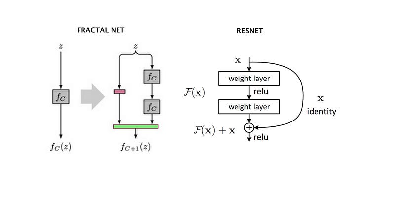
Regardless of the architectural designs of these networks, they all try to create channels for information to flow between the initial layers and the final layers. DenseNets, with the same objective, create paths between the layers of the network.
Related works
- Highway networks (one of the first attempts at making training easy for deeper models)
- ResNet (Bypassing connections by summation using identity mappings)
- Stochastic depth (dropping layers randomly during training)
- GoogLeNet (inception module — increasing network width)
- FractalNet
- Network in Network (NIN)
- Deeply Supervised Network (DSN)
- Ladder Networks
- Deeply-Fused Nets (DFNs)
Dense connections
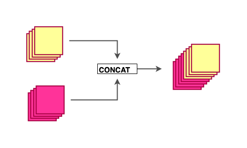
Following the feed-forward nature of the network, each layer in a dense block receives feature maps from all the preceding layers, and passes its output to all subsequent layers. Feature maps received from other layers are fused through concatenation, and not through summation (like in ResNets).
These connections form a dense circuit of pathways that allow better gradient-flow.
Each layer has direct access to the gradients of the loss function and the original input signal.
Because of these dense connections, the model requires fewer layers, as there is no need to learn redundant feature maps, allowing the collective knowledge (features learnt collectively by the network) to be reused. The proposed architecture has narrow layers, which provide state-of-the-art results for as low as 12 channel feature maps. Fewer and narrower layers means that the model has fewer parameters to learn, making them easier to train. The authors also talk about the importance of variation in input of layers as a result of concatenated feature maps, which prevents the model from over-fitting the training data.
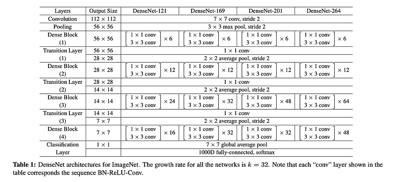
Many variants of the DenseNet model have been presented in the paper. I have opted to explain the concepts with their standard network (DenseNet-121).
Composite function
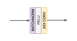
*Each CONV block in the network representations in the paper (and in the blog) corresponds to an operation of —
BatchNorm→ReLU→Conv*
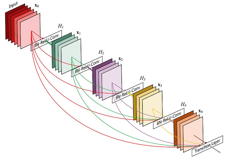
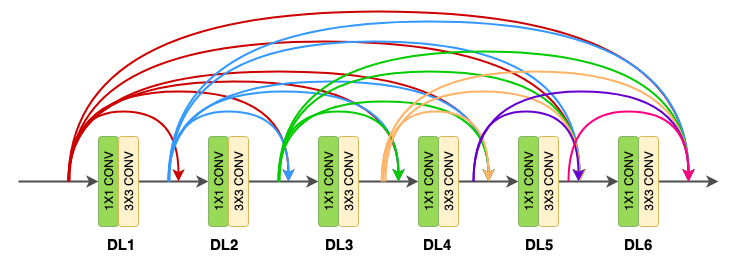
Dense block
The concept of dense connections has been portrayed in dense blocks. A dense block comprises n dense layers. These dense layers are connected using a dense circuitry such that each dense layer receives feature maps from all preceding layers and passes it’s feature maps to all subsequent layers. The dimensions of the features (width, height) stay the same in a dense block.
Dense layer
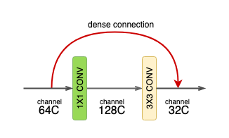
Each dense-layer consists of 2 convolutional operations -
- 1 X 1 CONV (conventional conv operation for extracting features)
- 3 X 3 CONV (bringing down the feature depth/channel count)
The DenseNet-121 comprises of 6 such dense layers in a dense block. The depth of the output of each dense-layer is equal to the growth rate of the dense block.
Growth rate (k)
This is a term you’ll come across a lot in the paper. It is basically the number of channels output by a dense-layer (1x1 conv → 3x3 conv). The authors have used a value of k = 32 for the experiments. This means that the number of features received by a dense layer ( l ) from it’s preceding dense layer ( l-1 ) is 32. This is referred to as the growth rate because after each layer, 32 channel features are concatenated and fed as input to the next layer.
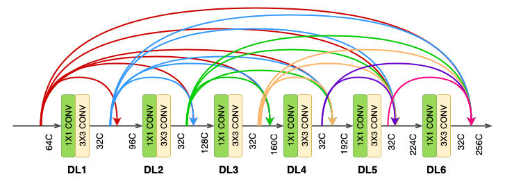
Transition layer
At the end of each dense block, the number of feature-maps accumulates to a value of — input features + (number of dense layers x growth rate). So for 64 channel features entering a dense block of 6 dense-layers of growth rate 32, the number of channels accumulated at the end of the block will be —
64 + (6 x 32) = 256. To bring down this channel count, a transition layer (or block) is added between two dense blocks. The transition layer consists of -
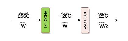
- 1 X 1 CONV operation
- 2 X 2 AVG POOL operation
The 1 X 1 CONV operation reduces the channel count to half.
The 2 X 2 AVG POOL layer is responsible for downsampling the features in terms of the width and height.
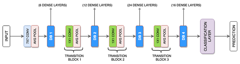
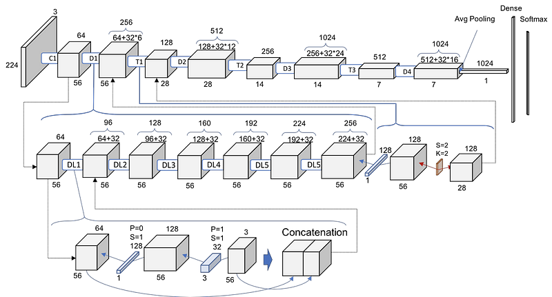
Full network
As can be seen in the diagram below, the authors have chosen different number of dense layers for each of the three dense block.
Comparison with DenseNet
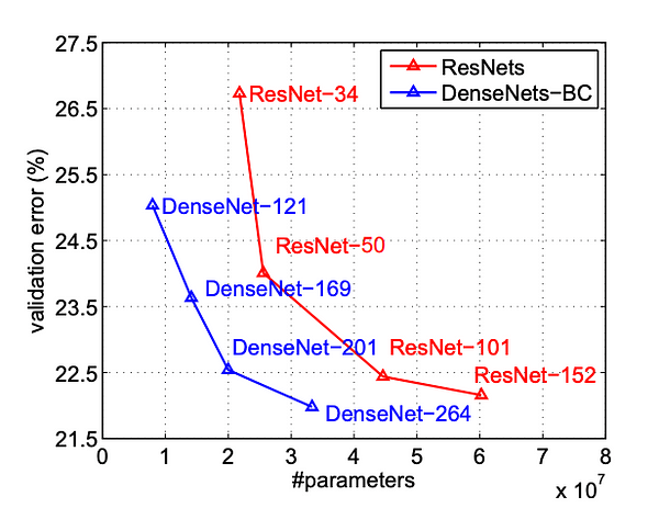
We can see that even with a reduced parameter count, the DenseNet model has a significantly lower validation error for the ResNet model with the same number of parameters. These experiments were carried out on both the models with hyper-parameters that suited ResNet better. The authors claim that DenseNet would perform better after extensive hyper-parameter searches.
DenseNet-201 with 20M parameters model yields similar validation error as a 101-layer ResNet with more than 40M parameters.
Inspecting the code
I believe that going through the code makes it easier to understand the implementations of such architectures. Research papers (in the context of Deep Learning) can be difficult to understand because they are more about what drives the design decisions of a neural network. Inspecting the code (usually the network/model code) can reduce this complexity because sometimes it’s just the implementation that we are interested in. Some people prefer first seeing the implementation and then trying to figure out the reasoning behind the design decisions of the network. Regardless, reading the code, before or after, always helps.
The code of the DenseNet implementation can be found here. Since I am more comfortable with PyTorch, I’ll try to explain the PyTorch implementation of the model which can be found here. The most important file would be models/densenet.py, that hold the network architecture for DenseNet.
The code has been divided into these classes where each type of block is represented by a class.
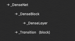
Dense layer
The _DenseLayer class can be used to initialise the constituent operations of a dense layer —
BatchNorm → ReLU → Conv (1X1) → BatchNom → ReLU → Conv (3X3)
The _bn_function_factory() function is responsible for concatenating the output of the previous layers to the current layer.
DenseBlock
The _DenseBlock class houses a certain number of _DenseLayers (num_layers).
This class is initialised from the DenseNet class depending on the number of dense blocks used in the network.
Transition Block
DenseNet
Since this part of the code is a little too big to fit in this blog, I’ll just be using a part of the code that should help in getting the gist of the network.
I found this image online and it has helped me understand the network better.
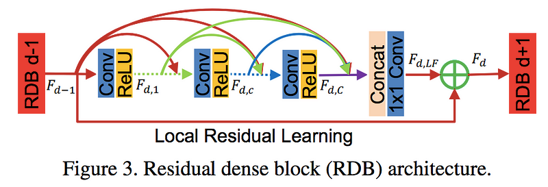
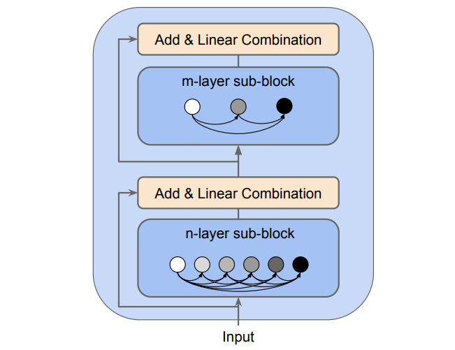
Other works inspired from this paper
Conclusion
DenseNet is a network that portrays the importance of having dense connections in a network using dense blocks. This helps in feature-reuse, better gradient flow, reduced parameter count and better transmission of features across the network. Such an implementation can help in training deeper networks using less computational resources and with better results.